Graphs are an excellent method to represent connections between items. A common example of graphs is users on a social network. A user is a node and the friendship is a connection. The world wide web is another common example; pages are nodes and hyperlinks are connections.
Graphs are made up of vertices and edges - vertices being the nodes in the graph, edges being a connection between a pair of vertices.
Graph Properties
Graphs come with a large corpus of definitions. The most common terms are briefly explained here.
A weighted graph is a graph with edges that have a numerical value associated with them.
A directed graph contains edges that have a head (the starting vertex) and a tail (the ending vertex of the edge)
Graphs can be a combination of weighted vs unweighted and directed vs undirected.
A graph is dense if the number of edges is close to the number of vertices. There is no hard rule as to what makes a graph dense though. The opposite of a dense graph is a sparse graph, meaning it has relatively few edges in comparison to the number of vertices in the graph.
An adjacency or path is an immediate edge between two neighboring vertices. Vertices are simply connected if they are apart the of the same graph, but not adjacent to each other.
The degrees is the number of edges a vertex has
Graphs that have have cycles, that is a connected component with continuous loop, are considered cyclic
As an aside, trees are special subset of graphs; they are directed acyclic graphs, otherwise known as a DAG.
A cycle is paths that start at vertex and end at the same vertex with 0 to n vertices included in the cycle.
Representing Graphs with Data Structures
Dictionaries
The simplest way to represent a graph is with a hashtable/dictionary/etc.
unweighted = {
    'A': {'B', 'C'},
    'B': {'A', 'D', 'E'},
    'C': {'A', 'F'},
    'D': {'B'},
    'E': {'B', 'F'},
    'F': {'C', 'E'}
}
The keys are vertices. Being that the above graph is unweighted, we simply store the adjacencies in a set as each key’s value.
Similarly, representing a weighted graph:
weighted = {
    'A': {'B': 5, 'C': 2, 'D': 3},
    'B': {'A': 5, 'D': 4},
    'C': {'A': 2, 'E': 1},
    'D': {'A': 3, 'B': 4},
    'E': {'C': 1}
}
Again, keys are vertices and values are key value pairs as adjacencies with weights associated with them.
While dictionaries are very straight-forward, it’s helpful to know there are other methods to store graph data.
Adjacency Matrix
Adjacency matrices are two-dimensional arrays that are size V² where V equals the total vertices in the graph.
A vertex list is used to tie keys to array indices. The vertex list is used as a map in the adjacency matrix to connected keys.
For unweighted graphs, the cells of the adjacency matrix are filled on a binary basis; a 1 to signify an adjacency and a 0 to signify no connection.
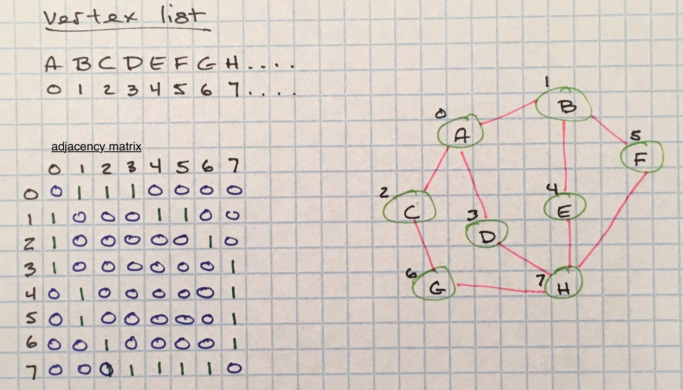
This representation can be used for weighted graphs as well, with weights used to represent adjacencies instead of 1.
While adjacency matrices are a simple, elegant way to represent connections in a graph, there tends to be a lot of wasted space if the graph is sparse. We are using a matrix to detail many non-existant connections.
It also adopts the benefits and trade-offs associated with using two-dimensional arrays to store data. Such as:
- space complexity being
O(V²). - querying if two vertices are connected is
O(1). - finding adjacent vertices for a specific vertex is
O(v). We first have to scan the vertex list for the index, access that index on the adjacency matrix, then linearly scan through that row to find all1’s (or weights).
Most real-world graphs are sparse, so using an adjacency matrix is pretty inefficient.
Adjacency Lists
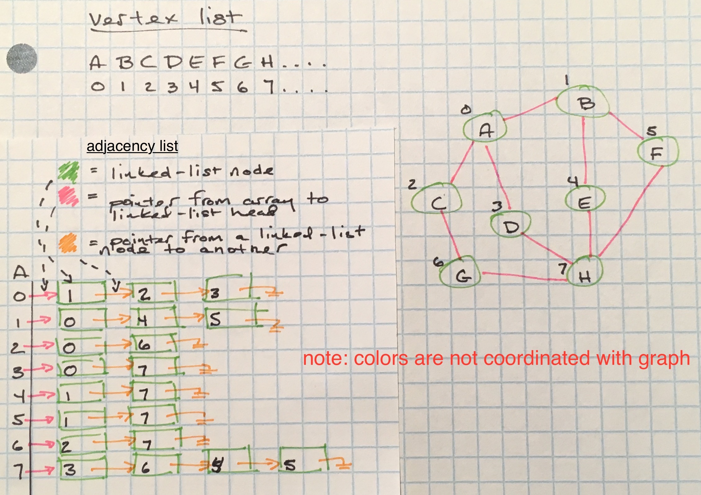
Adjacency lists are a space-efficient way to represent a sparse graph - their space complexity is O(E), E being the total edges in the graph.
Adjacency lists are not really lists, but rather mappings. The map a vertex list, (like what’s used in the adjacency matrix) to map node keys to indices in an array. Those array positions hold another data structure that will keep track of edges. Possible data structures that can be used to keep track of those edges are linked lists, hashmaps, a binary search tree, set, and arrays.
For the sake of simplicity, instead of using adjacency matrices or lists, I will use a hashmap for the rest of this post.
Determining Connected Components
One of the fundamental operations to use on an graph is determining what nodes are connected to a specific node. Otherwise known as determining a connected component.
From a starting vertex, neighboring vertices that have direct and indirect edges to the starting vertex are collected.
There are two ways to go about travering edges: depth-first and breadth-first.
Depth-First Traversal
Depth-first will visit a neighboring vertex and go deeper down its branches to its neighbors, until it has to backtrack where there no more edges.
def dfs(graph, start):
    visited, stack = set(), [start]
    while stack:
        vertex = stack.pop()
        if vertex not in visited:
            visited.add(vertex)
            to_be_visited = graph[vertex] - visited
            stack.extend(to_be_visited)
    return visited
Depth-first search can be implemented in an iterative fashion, but because it uses a stack as its underlying data structure, we can take advantage of the call stack and implement a recursive version as well:
def dfs(graph, vertex, visited=None):
    if visited == None:
        visited = set()
    visited.add(vertex)

    for neighbor in graph[vertex]:
        if neighbor not in visited:
            dfs(graph, neighbor, visited)
    return visited
Regardless of the implementation, the basic steps are:
- visit a vertex and mark it has having been visited (this prevents an infinite loop)
- visit all the vertices that are adjacent to it have not yet been marked
- repeat for each unvisited vertex
DFS will traverse each edge in connected component twice, and always finding a marked (visited) vertex the second time.
Breadth-First Traversal
As the name implies, instead of going deeper per branch, bread-first traversal finds all adjacencies to a vertex before it starts traversing deeper branches. Adjacencies at distance k are found before those at distance k+1.
Breadth-first uses a queue to store vertices that will eventually be visited, where their adjacencies will be queued up for eventual visiting, if they have not been visited yet.
Because BFS uses a queue as its underlying data-structure, implementing it in a recursive fashion is somewhat trickier. Here’s the iterative approach:
from collections import deque

def bfs(graph, start):
    visited, queue = set(), deque([start])
    while queue:
        vertex = queue.popleft()
        if vertex not in visited:
            visited.add(vertex)
            to_be_visited = graph[vertex] - visited
            queue.extend(to_be_visited)
    return visited
Path Finding
In addition to determining connected components, depth-first and breadth-first approaches can be used to find a path from a starting vertex to a goal vertex.
Breadth-First Path Finding
from collections import deque

def bf_paths(graph, start, goal):
    """first returned path is the shortest path"""
    if start == goal:
        yield [start]
        return

    queue = deque([(start, [start])])
    while queue:
        vertex, path = queue.popleft()
        to_be_visited = graph[vertex] - {path}
        for neighbor in to_be_visited:
            if neighbor == goal:
                yield path + [neighbor]
            else:
                queue.append((neighbor, path + [neighbor]))

def shortest_path(graph, start, goal):
    """retrieve only the shortest path from the path queue"""
    try:
        return next(bf_paths(graph, start, goal))
    except StopIteration:
        return None
For breadth-first, switching from determining connected components to finding paths requires is as easy as using this simple trick: cache the current path along with the vertex, and add vertices to the queue as the algorithm continues.
Breadth-first is useful for finding the shortest path from start to finish in an unweighted graph (if the graph is weighted, using Dijkstra’s algorithm is more appropriate - more on this below).
Depth-First Path Finding
def df_paths(graph, start, goal, path=None):
    if path is None: path = [start]

    if start == goal:
        yield path
        return

    for next_vertex in graph[start] - {path}:
        yield from df_paths(graph, next_vertex, goal, path + [next_vertex])
    }
A Depth-first path search is more applicable if you are looking for a goal vertex that is believed to be far away from the starting vertex. This is because DF goes deep per branch.
Path Finding in Digraphs
Path finding in digraphs can also use BF and DF.
The only difference is how the data is stored in a hashmap. Undirected graphs have edges saved for both vertices. This is not the case for digraphs; the hashmap will store the tail vertex in the set of values for a particular key, or head vertex.
Topological sort
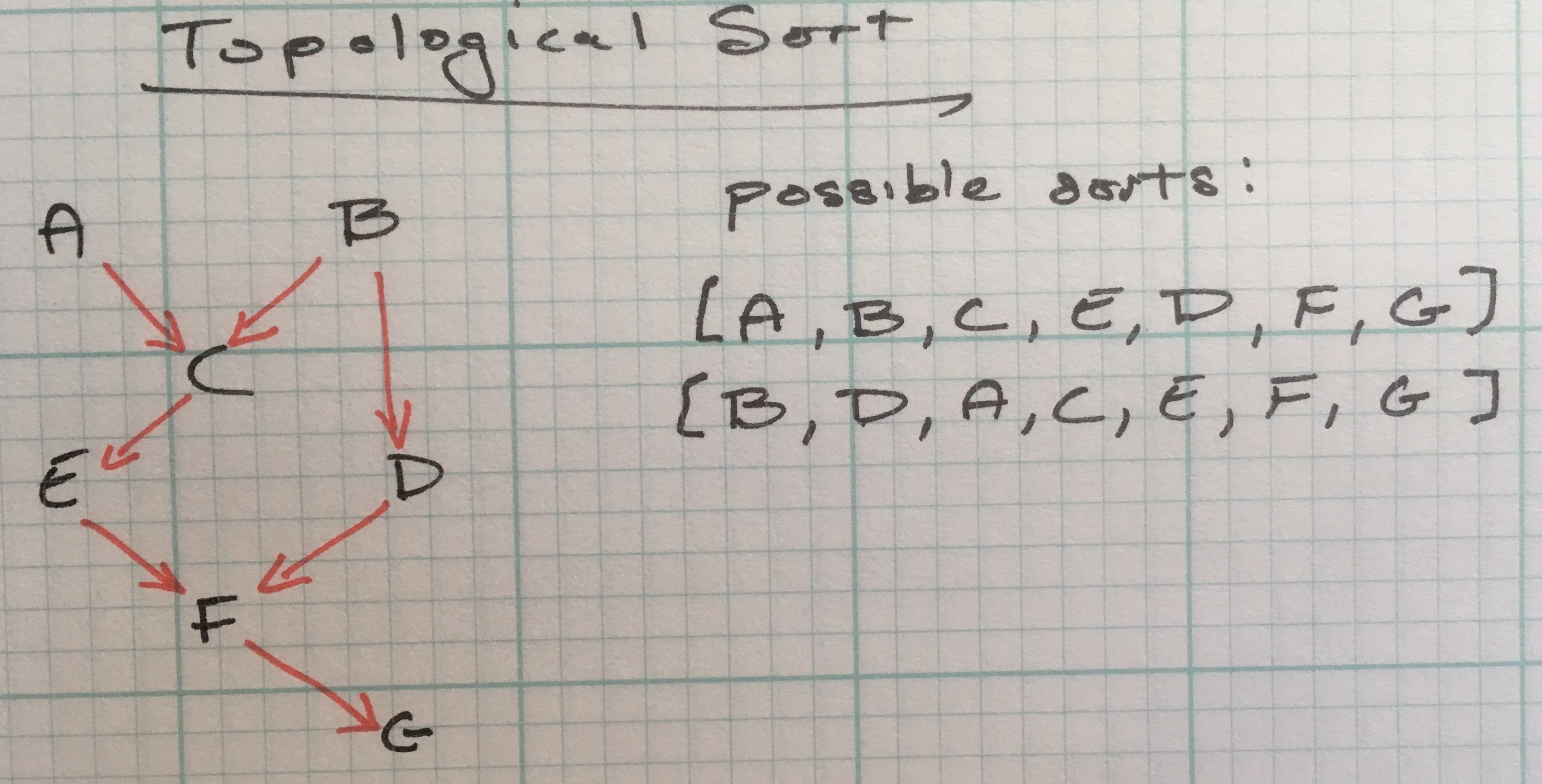
While graphs can have cycles, certain algorithms expect a graph to be acyclic.
The topological sort is one of these algorithms and its important for structuring vertices in a linear order. It relies on a directed acyclic graph.
Examples of where a topological sort is useful:
- Scheduling. Appointments are supposed to happen in a sequential order. How can we determine the order of a schedule for the day?
- Module loaders. Which module is the first module to load? How do we determine the order of the modules that need load after the first module?
Checking for cycles is important for topological sorts because it indicates there’s a mistake. If job x needs to complete before job y, and job y before job z, but job z is visited before job x, something is broken. If the digraph has a cycle, it’s not a topological sort.
def topological_sort(graph):
    visited, reversePostOrder = set(), deque()
    for head in graph:
        if head not in visited:
            dfs(graph, head, visited, reversePostOrder)
    return reversePostOrder


def dfs(graph, vertex, visited, reversePostOrder):
    if vertex not in visited:
        visited.add(vertex)
        for node in graph[vertex]:
            dfs(graph, node, visited, reversePostOrder)
        reversePostOrder.appendleft(vertex)
Dijkstra’s Algorithm and Weighted Graphs
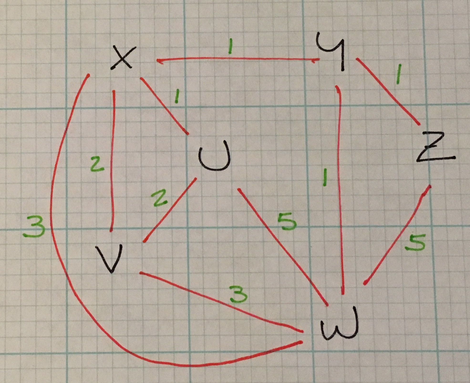
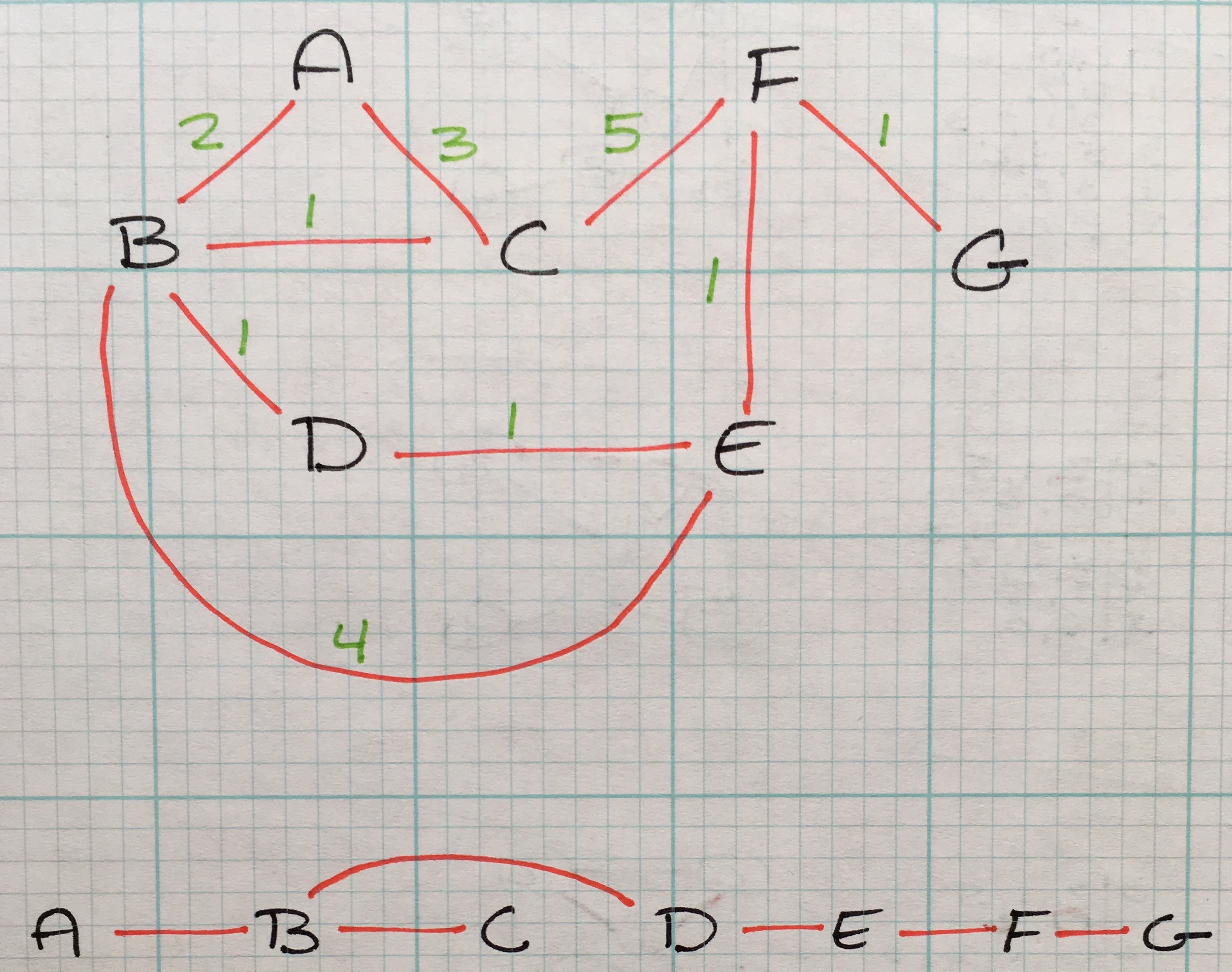
I hinted earlier in the explanation of breadth-first path finding that BF is useful for finding the smallest number of vertices between a start and end vertex and Dijktra’s algorithm is suited for finding cheapest route in a weighted graph.
What are some example of weighted graphs? + map of roads with weights as distances + an electrical circuit with wires representing cost or signal time
Back to Dijktra: in the above weighted graph, the algorithm would find the shortest path from Z to V is 4: (Z –1–> Y –1–> X –2–> V).
Dijktra is applicable to both directed and undirected graphs.
import heapq

def calc_distances(graph, starting_vertex):
    pq, distances = init(graph, starting_vertex)

    while pq:
        # pops off vertices in order of shortest distance from starting vertex
        current_distance, current_vertex = heapq.heappop(pq)

        for neighbor, neighbor_distance in graph[current_vertex].items():
            new_distance = distances[current_vertex] + neighbor_distance
            if new_distance < distances[neighbor]:
                # caches the shortest distance from current vertex to the adjacent vertex
                distances[neighbor] = new_distance

    return distances

def init(graph, starting_vertex):
    distances = {vertex: math.inf for vertex in graph}  # distances from starting_vertex to connected components
    distances[starting_vertex] = 0
    pq = [(distance, vertex) for (vertex, distance) in distances.items()]
    heapq.heapify(pq)

    return (pq, distances)
The algorithm keeps track of distances from a starting vertex using a hashmap. Keys are vertices in the graph and initial values are infinity, because we don’t know the distance from the starting vertex to a particular vertex. The exception is the key for the starting vertex, which is 0 because it’s, well, itself.
As the algorithm iterates through all the vertices, it updates the distance from starting vertex if it finds the current path is shorter than the previously cached path.
How does the algorithm determine the order of vertices to travel for the cheapest path? It uses a priority queue. By using a PQ, the vertex with the shortest path is continuously bubbled up to the top of the list after the previous vertex was popped off.
Some caveats about Dijktra:
- it only works for positive weights.
- it requires a complete representation of the graph in order to run (it cannot discover vertices as it goes).
It’s running time is O(V + E)log(V)).
Prim’s Algorithm
A similar algorithm to Dijktra is Prim’s algorithm, which is used to determine the cheapest way to connect all vertices in an graph. The data structure it creates is a minimum spanning tree.
minimum spanning tree T for a graph G = (V, E) is a acyclic subset of E that connects all the vertices in V.
Prim’s is a greedy algorithm - at each step it chooses the cheapest next step - in this case the cheapest next step is to follow the edge with the lowest weight, and adds that to the spanning tree.
Each vertex added to the spanning tree must not already be in the tree (again, it’s acyclic).
Like Dijktra, it uses a PQ to determine the next cheapest vertex to explore.
from collections import defaultdict
import heapq

def create_spanning_tree(graph, starting_vertex):
    mst, visited, edges = init(graph, starting_vertex)
    while edges:
        cost, frm, to = heapq.heappop(edges)
        if to not in visited:
            visited.add(to)
            mst[frm].add(to)
            for to_next, cost in graph[to].items():
                if to_next not in visited:
                    heapq.heappush(edges, (cost, to, to_next))
    return mst

def init(graph, starting_vertex):
    mst = defaultdict(set)
    visited = {starting_vertex}
    edges = [(cost, starting_vertex, to) for (to, cost) in graph[starting_vertex].items()]
    heapq.heapify(edges)
    return (mst, visited, edges)